In this post, I’ll show some of our scene capture results. I’ll also briefly talk about the exposure correction steps that went into these results.
These results were captured using Google’s Project Tango Tablet. The characteristics of the Tango tablet and the basic capture process will be described in the next post.
These scans were all captured in about 10 minutes each. The results shown are generated mostly automatically, with the only manual step being the removal of some bad image frames (which could easily be done automatically).
Results
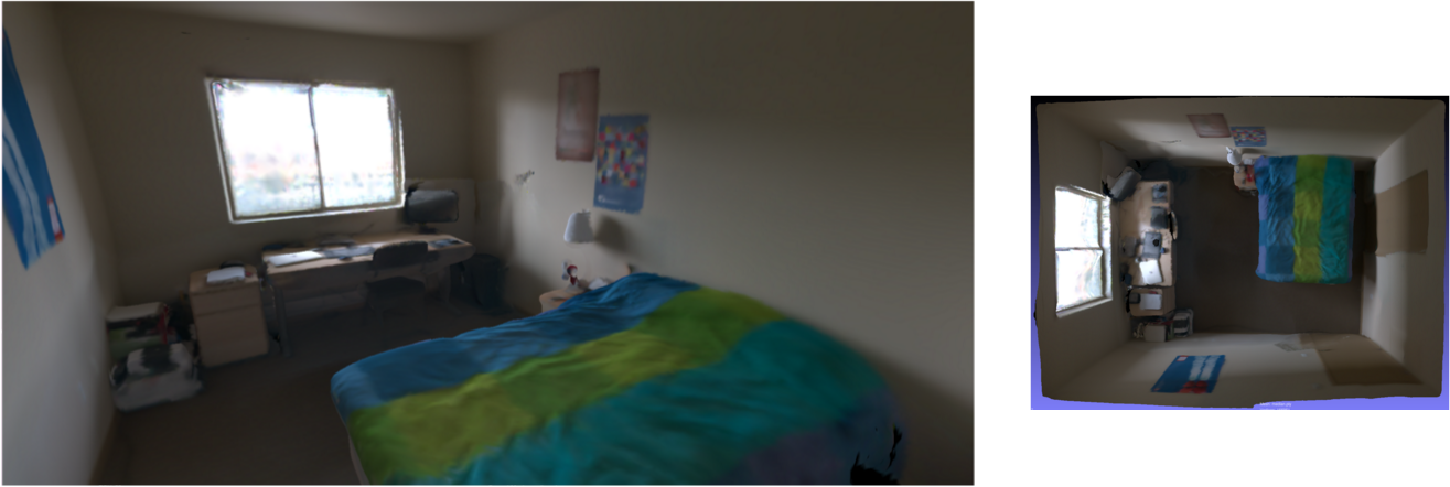
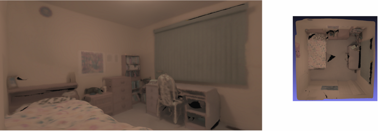
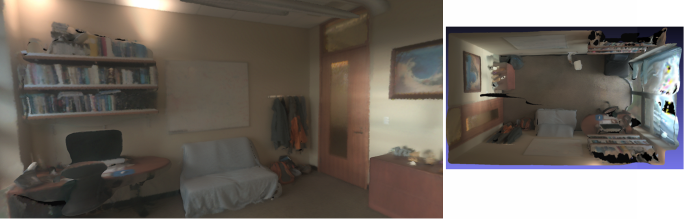
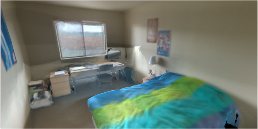
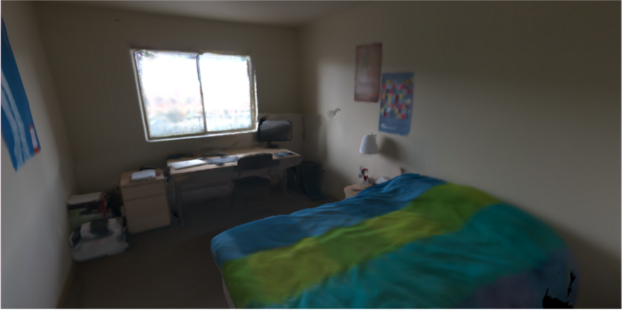
The following results are all screenshots taken in Meshlab of meshes with per-vertex colors (i.e. no textures). On the left is a view taken from inside the room, while the right has a top view of the scene. Below there is a Sketchfab embed for viewing the mesh. Linear tonemapping is applied to the mesh colors, as well as a gamma transform for viewing.
High Dynamic Range
Note that all of our results are in high dynamic range.
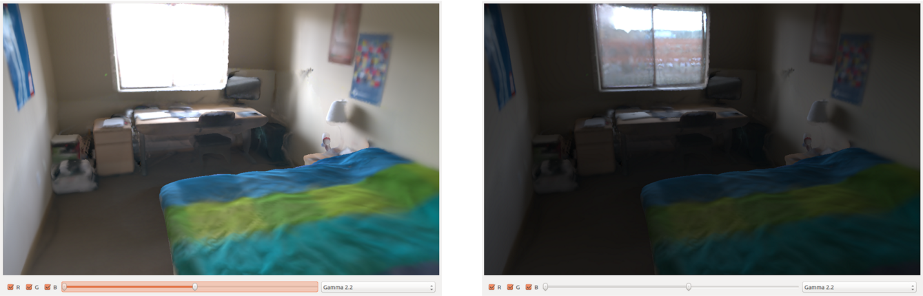
To obtain these results, we must perform radiometric calibration on the input frames. Without our radiometric calibration pipeline, we get low quality, low dynamic range meshes.
Radiometric Calibration
The images provided by most cameras, including the Tango, usually have autoexposure and auto-white-balance applied for optimal image quality. Unfortunately, this results in inconsistent appearance when the images are combined on the scene geometry. Our problem is basically to undo autoexposure, i.e. obtain a per-frame exposure time that lets us put the images into one common reference space.
Fortunately, this problem is fairly well understood in many contexts. The formulation most similar to ours is the one commonly used in panorama stitching.
Exposure correction in panorama stitching goes something like this:
- Find correspondences in the images.
- Warp the images and project them into a new coordinate space so that correspondences overlap. This puts pixels of images into dense correspondence
- Each set of pixels in the original images that map to the same warped coordinates should have the same “true” radiance value (which is unknown); any difference in pixel value should just be due to per-frame camera effects (i.e. exposure)
- Jointly optimize both the set of “true” radiance values and the per-frame exposures by minimizing the difference between each original image pixel (tranformed by the frame’s exposure) and its “true” radiance.
Mathematically,
- Let the camera response function \(f(b,t)\) map radiance \(b\) to a (0-255) pixel value given an exposure time \(t\).
- Let frame \(i\) have exposure time \(t_i\)
- Let point \(j\) in the final panorama space have an unknown true radiance \(b_j\).
- Let \(x_{ij}\) be the value of the pixel in image \(i\) that maps to point \(j\) in the final panorama space.
Then we want to optimize \(\min_{t_i,b_j}\sum_{i,j}{(f(b_j,t_i) - x_{ij})^2}\)
Fun tidbit - this formulation is identical to the Bundle Adjustment formulation used in Structure from Motion. This means we can use the many tools and methods used in bundle adjustment to solve this optimization problem robustly and efficiently. In practice, we just toss everything into Ceres Solver and let it work its magic.
Of course, we can’t just directly apply the panorama stitching methods to our task. With our moving camera, the parallax caused from nearby objects means that simple image warps are not going to globally align our frames very effectively. Instead, we make use of the scene geometry and camera poses we have.
Now, instead of warping images, we project them onto the scene geometry. Each set of pixels in the original images that map to the same mesh vertex should have the same “true” radiance value (given a Lambertian assumption). Then we can proceed with the bundle adjustment as usual. In our results, we have a simple linear camera response (after gamma correction) \(f(b,t) = tb\), and we just use the L2 norm as illustrated above.
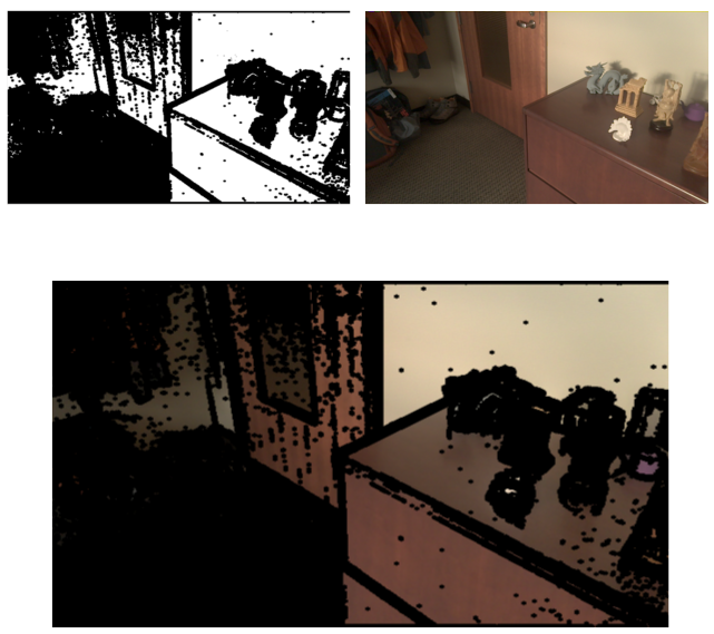
One last detail: To make our solution cleaner, we want to throw away as many bad correspondences as possible. Bad correspondences will usually occur near depth discontinuities, where even minor misregistrations will put pixels from one object onto another one. So when projecting, we mask out pixels near edges to minimize this effect.