The idea for this post was written after some people asked what my previous post and spherical harmonics were all about. This is my attempt at explaining them in a visually interesting, intuitive fashion.
Functions
Let’s start with functions. Functions map values from a domain to a range. Let’s see some examples:
- The typical 1D function covered in high school algebra goes from real-valued scalars to real-valued scalars: \(f: \mathbb{R} \rightarrow \mathbb{R}\). Visualizing these functions is done as a line on a 2D Cartesian plane, with domain on the x-axis and range on the y-axis.
- Another type of 1D function are those defined as polar functions: \(f: [0, 2\pi) \rightarrow \mathbb{R}\). Visualizing these functions is done as a line on a polar plot, where the domain is the angle relative to the horizontal axis and the range is the distance from the origin.
-
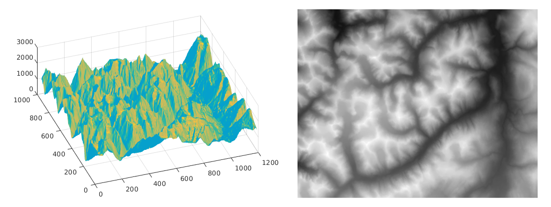
A typical 2D function, \(f: \mathbb{R}^2 \rightarrow \mathbb{R}\) can be analogously visualized as a surface in a 3D Cartesian space, with domain on the x- and y-axes, and range on the z-axis.
-
However, we can also represent a 2D function in two dimensions, by using x- and y-axes as domain and intensity as range. In other words, a grayscale image is a 2D function. One caveat: negative function values obviously can’t be represented as a physical intensity, so to deal with negative values in 2D functions, we need to e.g. show negative values in a different hue than positive values.
- Our image representation naturally extends itself to a higher dimensional range: a (nonnegative) function \(f: \mathbb{R}^2 \rightarrow \mathbb{R}^3\) can be visualized as a color image, with the red, green, and blue components being the first, second, and third coordinates of the range.

- A more interesting set of functions are those defined on the spherical domain, \(f: (\theta \in [0, \pi], \phi \in[0, 2\pi)) \rightarrow \mathbb{R}\). Spherical functions are to 2D functions as polar functions are to 1D functions.

Function Approximation
General functions are hard to deal with for practical purposes, since they can be defined arbitrarily. You might have a nice polynomial function \(f(x) = ax^2 + bx + c\), or it might use some less well-known function like \(f(x) = \sinh(x)\), or it could just be an infinite lookup table of values. For real world applications, there is often no way to write down the function precisely - the price of a stock as a function of time, the temperature as a function of location on the earth, and so on.
So when modelling real-world phenomena, we approximate functions by putting them into some more natural representation. There are many ways of doing this: you can fit a function to it, use a deep neural network, a support vector machine, and so on. Here, we’re going to represent functions as linear combinations of basis functions. What does this mean? Basis functions are just a set (possibly infinite) of pre-defined functions that are defined on the same domain as the function we want to represent. We form a linear combination of these functions by multiplying each of them by a different coefficient and then add them all up. So the representation of our original function \(f(x)\) becomes simply the set of scale factors (coefficients) \(c_i\) of our basis functions \(b_i(x)\).
\[f(x) = c_1b_1(x) + c_2b_2(x) + ... + c_nb_n(x) = \sum c_ib_i(x)\]See the figure below for some visual examples.
Linear Bases
Here we’ll go over some common types of basis functions. These function types generalize to many different domains; here we’ll show examples for approximating a 1D function and a 2D function.
| Basis Function | 1D basis functions | 1D reconstruction |
|---|---|---|
| Constant Basis | 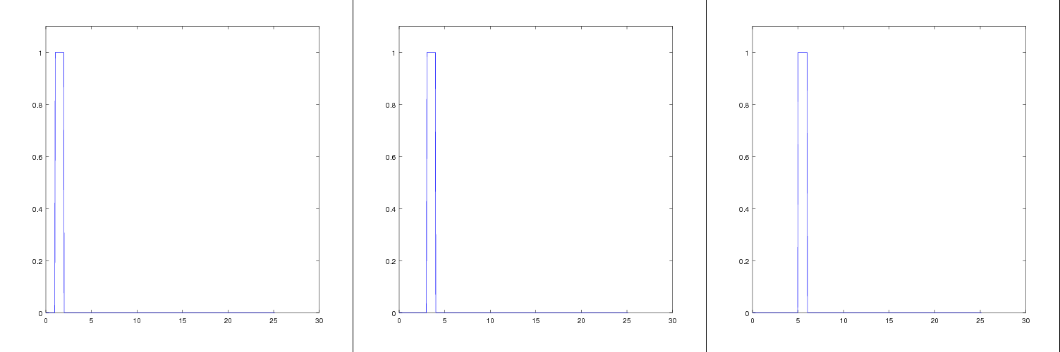
|
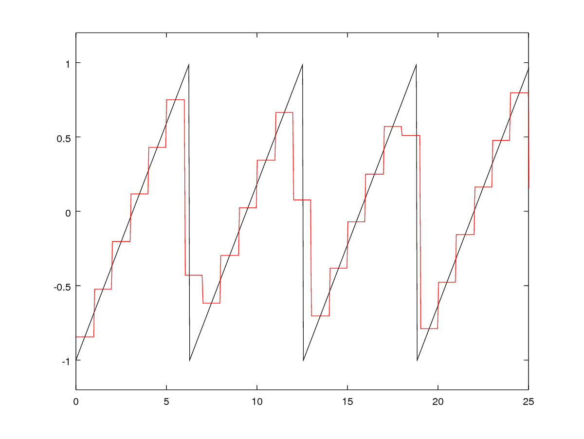
|
| Radial Basis | 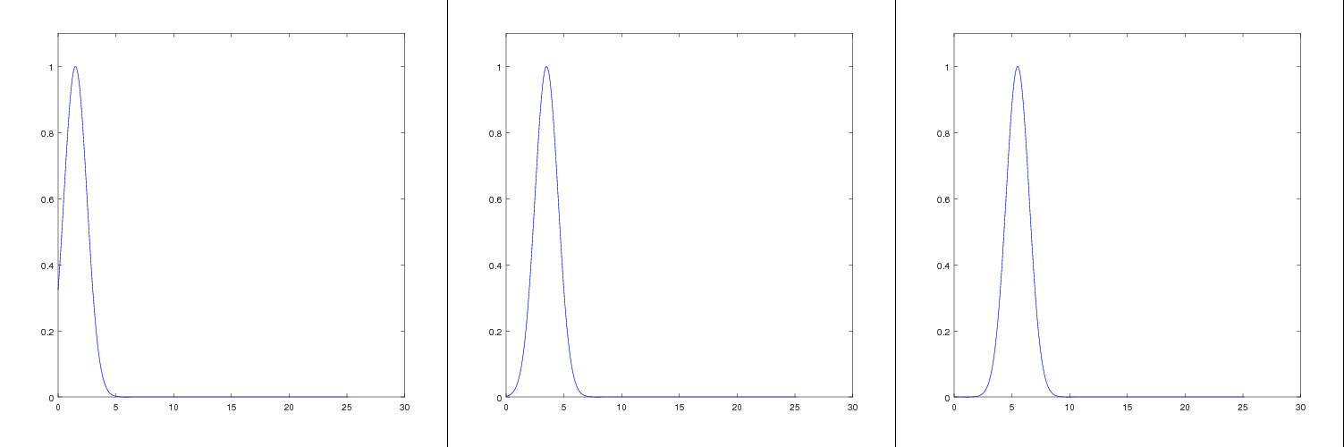
|
|
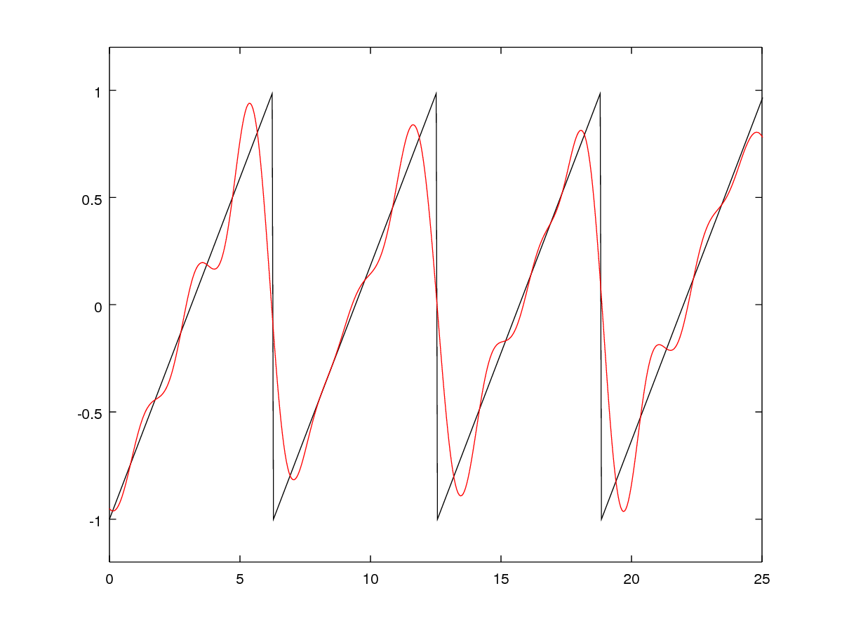
| Harmonic Basis | 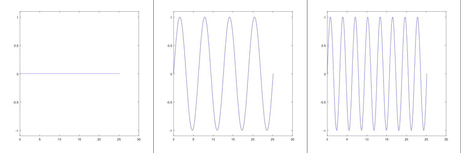
|
|
| Wavelet Basis | 
|
|
| Polynomial Basis | 
|
|
| Basis Function | 2D basis functions
| 2D reconstruction
|
|---|---|---|
| Constant Basis | 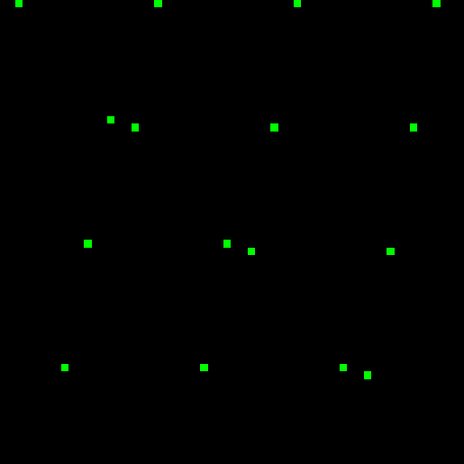
|

|
| Radial Basis | 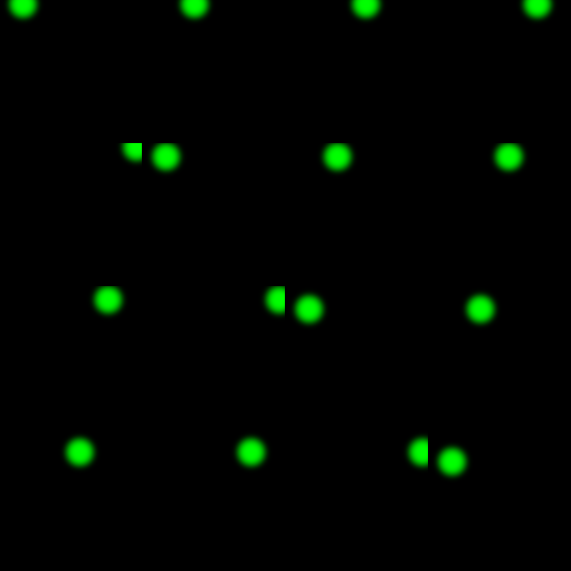
|

|
| Harmonic Basis | 
|

|
| Wavelet Basis | 
|

|
| Polynomial Basis | 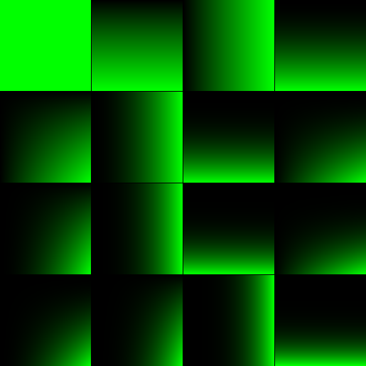
|

|
-
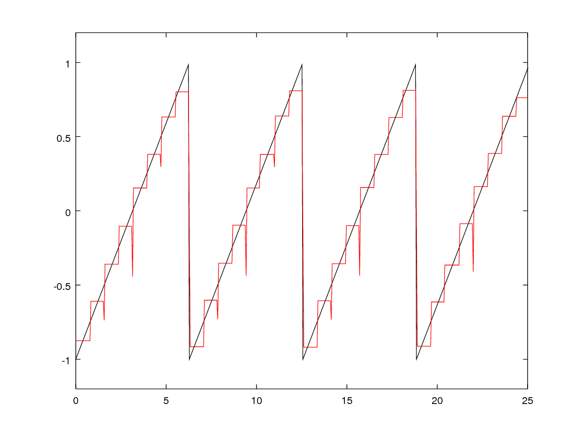
The constant basis is a very simple one. You split the domain into discrete sections; each basis function is 1 within the section and 0 everywhere else. Pixel-wise representation of images are constant basis representations, as are digital audio signals. The constant basis is very general for finite domains, and is easy to compute (each coefficient only depends on the function’s values within each section, i.e. it is locally supported). It usually results in significant aliasing (jaggy edges) if used naively.
-
Closely related to the constant basis is the radial basis. In radial basis functions, you pick a set of “centers” in your domain; each basis function has a peak at the center and smoothly falls to zero not too far from the center. Usually, Gaussian functions are used as the basis functions. RBF reconstructions of functions are smoother than constant basis representations, but otherwise have similar benefits and drawbacks.
-
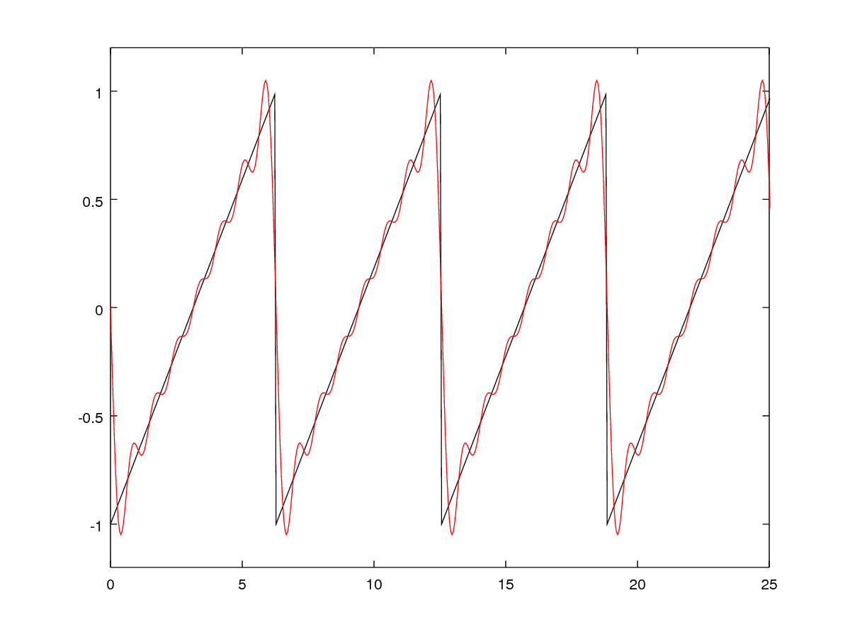
The harmonic basis (such as the 1D Fourier basis) is a more theoretically motivated set of basis functions. In 1D, the basis functions are simply \(\sin(x), \sin(2x), \sin(3x)... \sin(nx)...\). Technically, the Fourier basis isn’t quite a linear basis, since the coefficients may be complex (the imaginary component encodes the phase); the Discrete Cosine (or Sine) Transform is the simpler version in real numbers only. This basis has the very nice property that using only the first few basis functions usually results in a pretty good approximation of the function; in signal-processing terms, they encode the low frequencies of the function. Harmonic bases are nonlocal, in that changing the function values in one place changes all the coefficients.
-
A wavelet basis is similar to the Fourier basis in that it captures different signal frequencies in different basis functions; however in a wavelet basis, higher order basis functions are more localized over the domain. Haar wavelets are the most common example of wavelets.
-
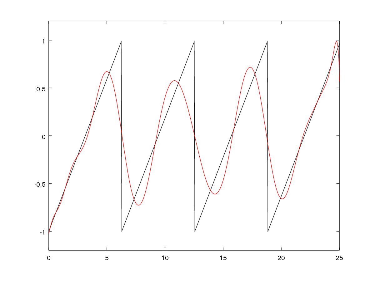
Another basis that is commonly used is the polynomial basis. When you do a polynomial fit in Matlab, you are finding a representation in the polynomial basis. When you do a Taylor expansion of a function, you’re also getting a polynomial basis representation. The basis functions are the polynomials; for 1D they are \(1, x, x^2, x^3...x^n...\) while for 2D they are \(1, x, y, x^2, 2xy, y^2, x^3, 3x^2y, 3xy^2, y^3... \{(x+y)^n\}...\) (the constant factors are included for illustrative purposes, but not actually used). For most applications, we only take the linear or quadratic approximation since it’s much easier to analyze and work with. Like the harmonic basis, the polynomial basis is nonlocal.
Back to Spherical Harmonics
Armed with this knowledge, spherical harmonics are now easy to define. They are simply the set of harmonic basis functions over the spherical domain. This is what the spherical harmonic basis functions look like:
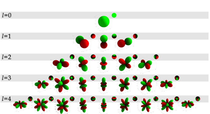
The spherical harmonic functions are referenced by two indices, usually \(l, m\). \(l\) is referred to as the band, while \(m\) is sometimes called the index. \(l\) corresponds to the frequency of the signal (e.g. band 0 is the bias, band 1 is very low frequency, and adding more bands adds higher frequencies). \(m\) ranges from \(-l\) to \(l\) in each band, so that using an \(n\)-band spherical harmonic approximation results in \(n^2\) basis functions.
Spherical harmonics in computer graphics and vision are commonly used to represent incident lighting: if you consider a point on a surface, the intensity of the light hitting it is a function of direction. It has been shown that, for diffuse surfaces, three bands (i.e. nine coefficients) of incident lighting spherical harmonics are indistinguishable from higher frequency representations of the incident light. The diffuseness of the surface essentially blurs out the higher frequencies.
If you’ve ever seen diagrams of electron orbitals, they happen to have the exact same shape as the spherical harmonics! More precisely, the solution to the Schrodinger Equation for a hydrogen atom are multiples of the spherical harmonics (see Wikipedia).
I won’t go into any of the mathematical details behind the functions; if you do need more depth, a list of references is at the end of this page.
Working with Linear Bases
There are many things you can do using linear bases; “function approximation” is a very broad term. What we did above can be seen as compression: we took a dense sampling of a function, and then represented it with a much smaller number of coefficients. In the sawtooth case, we took 512 samples of a sawtooth function and compressed it into 32 or fewer numbers; in the image case we took \(128 \times 128 = 16384\) pixels and represented them with 225 numbers or fewer.
We can also use linear bases for interpolation: if we only had a sparse sampling of function values, and we want to know the function value for somewhere we don’t have a value for, we can just use the linear basis approximation.
In both of these cases, we want to use a sampling of function values, and project the function into the linear basis. The most general way to do this is, unsurprisingly, linear least squares. Given a list of \(m\) observations \((x_j, f(x_j))\), you can form the equations
\(f(x_1) \approx \hat{f}(x_1) = c_1b_1(x_1) + c_2b_2(x_1) + ... + c_nb_n(x_1) = \sum_i c_ib_i(x_1)\)
\(f(x_2) \approx \hat{f}(x_2) = c_1b_1(x_2) + c_2b_2(x_2) + ... + c_nb_n(x_2) = \sum_i c_ib_i(x_2)\)
\(...\)
\(f(x_m) \approx \hat{f}(x_m) = c_1b_1(x_m) + c_2b_2(x_m) + ... + c_nb_n(x_m) = \sum_i c_ib_i(x_m)\)
You then want to minimize the squared differences between your observed values \(f(x_j)\) and your fitted values \(\hat{f}(x_j)\).
\[\min_{c_i} \sum_j \left( f(x_j) - \sum_i c_ib_i(x_j)\right)^2\]You can just plug in your values for \(f(x_j)\) and evaluate the \(b_i(x_j)\) (since you know your basis functions), so that your only unknowns are the \(c_i\).
Sample code for using linear least squares for function approximation (including code used to generate the above images) is available at https://github.com/kyzyx/linearbasis. Note that, while linear least squares will work for projecting into any linear basis, it is not always the most effective way to do so. For example, when using the harmonic bases, you usually want to use a Fourier transform instead; various types of wavelet transforms also exist for different types of wavelet bases.
You can do much more than just interpolation and compression with function approximation! What if you can’t actually directly get samples \((x, f(x))\) of your function? For example, in my research, I want to determine some unknown lighting distribution \(L(\phi, \theta)\), but I have no direct observations of \(L\). Instead, I only indirectly see the effects of the lighting by what the surfaces in the scene look like, e.g. \(B = \int_\Omega f(\omega) L(\omega) d\omega\), where the only things I know are \(B\) and maybe \(f\). By writing \(L\) as a linear combination of basis functions, we can optimize directly for the coefficients of \(L\) in the linear basis. This lets us get an approximation for the full function \(L\) without actually having seen any values for the function!
Conclusion
Linear bases are an extremely simple but powerful tool for function approximation. There are all sorts of theoretical pros and cons to the bases presented here that I haven’t gotten into (e.g. orthogonality, nonnegativity), but hopefully this gives you an intuitive sense as to how they work. If you were here just to figure out spherical harmonics, this might have been a rather roundabout and low-level way to explain them. If you want to dive more deeply into them, hopefully I’ve provided enough of the first principles to make the references below less confusing.
Spherical Harmonics References
Here are a collection of classic references for spherical harmonics, usually in the context of lighting.
- Spherical Harmonic Lighting: The Gritty Details: the authoritative reference for spherical harmonics in computer graphics.
- Stupid Spherical Harmonics (SH) Tricks: another commonly cited reference for spherical harmonics in computer graphics. Contains useful appendices, including polynomial approximations and code for up to 5 bands.
- In-Depth: Spherical Harmonic Lighting: a concise reference for SH lighting
- An Efficient Representation for Irradiance Environment Maps: the original paper by Ramamoorthi describing the use of spherical harmonics for diffuse environment maps
- On the relationship between radiance and irradiance: Math-heavy theoretical analysis by Ramamoorthi on diffuse SH lighting